Getting started with satpt

With the package installed and loaded into the current R environment, we may begin exploring the functionality of this package through examples.

library(satpt)
#> 
#> Attaching package: 'satpt'
#> The following object is masked from 'package:stats':
#> 
#>     simulate

Examples

Basic usage of `satpt`

To start, we will load in the example Difficult Diagnoses data to work with.

# Load diagnoses data
data(diagnoses)
str(diagnoses)
#> List of 3
#>  $ wave: num [1:643] 2 3 3 2 2 3 3 3 2 3 ...
#>  $ q1  : chr [1:643] "Broadrange|Wholegenome|MNGS" "Broadrange|Wholegenome|MNGS" "Broadrange|MNGS" "Broadrange" ...
#>  $ q2  : Factor w/ 5 levels "Not at all","Once",..: 4 5 4 2 3 3 3 3 4 4 ...

## Turn diagnoses data into data.frame
diagnoses <- do.call(what = "cbind.data.frame", args = diagnoses)

We will start by examining whether the responses collected in the second question (q2) of the diagnoses data achieved saturation.

levels(diagnoses$q2)
#> [1] "Not at all" "Once"       "Rarely"     "Sometimes"  "Often"

The res object below is a satpt object that contains the results of the saturation point analysis and is structurely a R list with twelve elements produced by main function satpt::satpt(). You may see the documentation of satpt::satpt() for a detailed description of all the elements of a satpt object.

res <- satpt::satpt(y = diagnoses$q2, threshold = 0.025)

For a basic examination of the saturation point analysis, you may simply print the results object. This will provide information of whether the maximum standard errors of the response categories are less than or equal to the saturation threshold along with sample proportions and standard errors of the response categories. In this example, the default saturation threshold of 0.025 was used and the maximum standard error was less than 0.025. Thus, saturation of the response categories is achieved.

print(res)
#> Analysis based on: q2 
#> Saturation achieved?  Yes 
#> 
#> Overall Sample Proportions and Standard Errors
#> ==============================================
#>             y: q2
#> Statistics   Not at all  Often   Once Rarely Sometimes
#>   Proportion     0.2531 0.0750 0.0375 0.3688    0.2656
#>   SE             0.0172 0.0104 0.0075 0.0191    0.0175

When a more detailed look at the analysis is warranted, simply call summary() on the returned satpt object, as seen below.

summary(res)
#> 
#> Saturation point analysis of sample proportions
#> ===============================================
#> 
#> Analysis based on: q2 
#> Saturation achieved? Yes
#> Saturation threshold of 0.025
#> Responses collected from a sample size of 640
#> 
#> Overall sample proportions
#> ============================================
#>          y: q2
#>           Not at all Often   Once Rarely Sometimes
#>   Overall     0.2531 0.075 0.0375 0.3688    0.2656
#> 
#> 
#> Overall standard errors
#> =========================================
#>          y: q2
#>           Not at all  Often   Once Rarely Sometimes
#>   Overall     0.0172 0.0104 0.0075 0.0191    0.0175

The goal of summary() is to provide a conditional comphrensive overview of the saturation point analysis similar in style to results produced by SAS procedures.

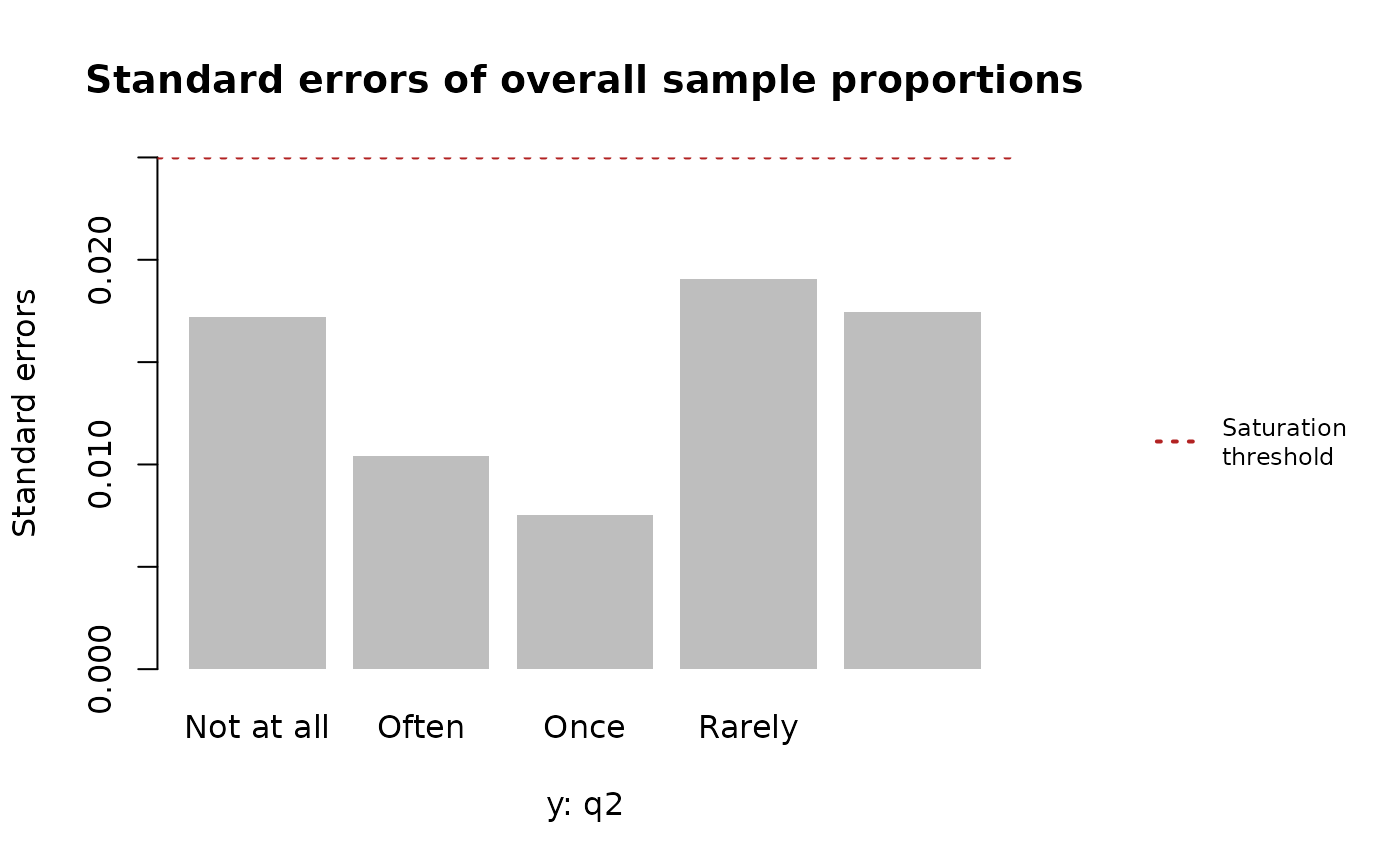
Another way of examining saturation point analysis is graphical by plotting the standard errors of the overall sample proportions for each response category in relation to the saturation threshold. With all the standard errors falling below the saturation threshold, we would say that we have achieved saturation for these responses.

graphics::par(oma = c(0, 0, 0, 8))
plot(res)
# adding legend
satpt::legend_right(
  legend = "Saturation\nthreshold",
  col = "firebrick", lty = 3, lwd = 2,
  cex = 0.75
)

Possibility of response bias

There will be times the data collection process leads to responses with the potential of having response bias. Thus, when performing saturation point analysis we must test for response bias and if response bias is present, we must account for that bias in the saturation point analysis. One example where response could be present is collecting data in waves based on non-responses in the previous waves. The diagnoses data previously explored was collected in this manner. Presented below is the number of responses collected for the second question for each data collection wave.

stats::ftable(x = diagnoses$wave)
#> x   1   2   3
#>              
#>   324 147 172

So, we are going to examine the responses collected in each wave for saturation, where the previous wave of responses will be included in the current wave and the saturation threshold is 0.025.

First data collection period

During the first data collection period, we are going to assume response bias is not possible because the responses were not collected due to non-responses in the previous wave, as there was no “previous” data collected.

# Subsetting the data to only include data collected during the first wave
diagnoses1 <- subset(x = diagnoses, subset = wave == 1)

# Performing saturation point analysis
res1 <- satpt::satpt(
  y = diagnoses1$q2,
  threshold = 0.025,
  dimnames = "Responses to survey"
)
print(res1)
#> Analysis based on: q2 
#> Saturation achieved?  No 
#> 
#> Overall Sample Proportions and Standard Errors
#> ==============================================
#>             y: Responses to survey
#> Statistics   Not at all  Often   Once Rarely Sometimes
#>   Proportion     0.2623 0.0833 0.0463 0.3364    0.2716
#>   SE             0.0244 0.0154 0.0117 0.0262    0.0247

Second data collection period

The results from the first data collection period show that saturation was not achieved, as the maximum standard error of the response items was not less than or equal to the saturation threshold. So, we’ll examine the data collected during the first and second data collection period for saturation of responses. For this analysis, we must account for the possibility of response bias by specifying the by argument in satpt::satpt() because the responses collected during the second wave include responses from EIN members who did not respond previously.

# Subsetting the data to only include data collected during the first and second
# waves of data
diagnoses2 <- subset(
  x = diagnoses,
  subset = wave %in% c(1, 2)
)

# Performing saturation point analysis
res2 <- satpt::satpt(
  y = diagnoses2$q2,
  by = diagnoses2$wave,
  threshold = 0.025,
  dimnames = c("by" = "Data collection period", "y" = "Responses to survey")
)
print(res2)
#> Analysis based on: q2 
#> Saturation achieved?  Yes 
#> 
#> Overall Sample Proportions and Standard Errors
#> ==============================================
#>             y: Responses to survey
#> Statistics   Not at all  Often   Once Rarely Sometimes
#>   Proportion     0.2596 0.0809 0.0426 0.3574    0.2596
#>   SE             0.0202 0.0126 0.0093 0.0221    0.0202

With the inclusion of the responses from the second data collection, saturation is achieved. We can take a look at the summary of the analysis, including the test of independence of the responses.

summary(res2)
#> 
#> Saturation point analysis of sample proportions
#> ===============================================
#> 
#> Analysis based on: q2 
#> Saturation achieved? Yes
#> Saturation threshold of 0.025
#> Responses collected from a sample size of 470
#> 
#> Data interval and overall sample proportions
#> ============================================
#>                           y: Responses to survey
#> by: Data collection period Not at all  Often   Once Rarely Sometimes
#>                    1           0.2623 0.0833 0.0463 0.3364    0.2716
#>                    2           0.2534 0.0753 0.0342 0.4041    0.2329
#>                    Overall     0.2596 0.0809 0.0426 0.3574    0.2596
#> 
#> 
#> Data interval and overall standard errors
#> =========================================
#>                           y: Responses to survey
#> by: Data collection period Not at all  Often   Once Rarely Sometimes
#>                    1           0.0244 0.0154 0.0117 0.0262    0.0247
#>                    2           0.0360 0.0218 0.0151 0.0406    0.0350
#>                    Overall     0.0202 0.0126 0.0093 0.0221    0.0202
#> 
#> Pooled standard errors?  No 
#> 
#>  Pearson's Chi-squared test
#> 
#> data:  y: Responses to survey given by: Data collection period
#> X-squared = 2.3255, df = 4, p-value = 0.6761
#> 
#> Response bias present? No
#> Significance level: 0.05
#> 
#> 
#> Heterogeneity index
#> ====================
#>  Categories  Index
#>  Not at all 0.0045
#>       Often 0.0040
#>        Once 0.0060
#>      Rarely 0.0338
#>   Sometimes 0.0194

The above Pearson’s \(\chi^{2}\) test for independence shows that responses bias was not present with a non-significant p-value. Thus, signifying the responses collected during the first and second data collection waves are not statistically different. With no response bias being present, traditional standard errors for the overall sample proportions of the response categories were calculated.

Saturation thresholds

The default saturation threshold in satpt::satpt() is 0.025 because this threshold for standard errors leads to a confidence interval width of 0.1 around the sample proportions. More specifically, for a \(95\%\) confidence interval around the sample proportions that has a margin of error (ME) of approximately

\[ ME = 1.96 \times \text{SE} = 0.05 \]

and a total width of 0.1, the saturation threshold, should be defined as 0.025. The table below provides more saturation thresholds based on confidence intervals that have a width of 0.1.

Confidence level	Saturation threshold
90%	0.038
95%	0.025
99%	0.210